Working paper · Version 2 · 35 pages
Order Book Imbalance and the Direction of the Next Mid-Price Change: Evidence from Nasdaq TotalView-ITCH
Posted: November 9, 2026
Abstract
We test whether order book imbalance, as computed by a commercial visualization application, predicts the direction of the next mid-price change. On four held-out days, under a pre-analysis plan fixed before their outcomes were computed, the sign of the reading matched the next change 55.1% of the time against a base rate of 50.0%, over 7,722,048 events among the 100 most active Nasdaq-listed stocks of each day. The relation is stronger at a one-tick spread, for lower-priced stocks and for mid-price changes that arrive soonest, as predicted, and it survives controls for the last mid-price change and recent signed volume.
1 Introduction
An order book imbalance summarizes the visible limit order book in one number: the size resting on the bid side minus the size resting on the ask side, divided by their sum. A positive reading says that more size waits to buy than to sell near the quotes. This paper asks whether such a reading, computed as a commercial order book visualization application computes it in the settings tested here (Section 3.3), predicts the direction of the next change in the mid price.
The question has a theoretical answer. When the bid-ask spread is one tick, the mid price moves only when one of the two best queues is exhausted, and a race between two queues tends to be lost by the shorter one (Avellaneda, Reed, and Stoikov (2011); Cont and de Larrard (2013)). Empirical work agrees. Book imbalances relate to short-horizon returns on the Australian Stock Exchange after controls for return autocorrelation, the spread and trade imbalance (Cao, Hansch, and Wang (2009)), order flow imbalance at the best quotes explains short-horizon price changes with a slope that falls with market depth (Cont, Kukanov, and Stoikov (2014)), and the imbalance of the two best queues predicts the direction of the next mid-price change on Nasdaq, most strongly for large-tick stocks (Gould and Bonart (2016)). The same quantity underlies the micro-price of Stoikov (2018) and the order book signals of Cartea, Donnelly, and Jaimungal (2018).
We study the imbalance reading of the VisualHFT application, a commercial order book visualization application, on Nasdaq TotalView-ITCH order-by-order data. In the settings we test, the reading weights each displayed level by its distance from its own side’s best quote and covers ten levels per side. These settings were selected on one day in an earlier study of the same feed, and we hold them fixed. Before any day was replayed for this study, we committed a pre-analysis plan that names the sample rule, the event definition, the hold-out days, six hypotheses with their specifications, the inference and every robustness check; we report each of them. The sample is the 100 most active Nasdaq-listed common stocks, by number of trades, selected afresh on each of seven full trading days between January 2019 and January 2020, and on a packet capture of 2023-08-22, which we report separately. Four of the seven days had never been replayed through the measure, and they form the hold-out.
On the four hold-out days, the sign of the first new reading after each mid-price change, which is the reading computed on the update that made that change whenever that update produced a new nonzero reading (Section 4.1), matched the direction of the next change 55.1% of the time, against 50.0% for a reading that carries no information about direction, a difference of 5.02 percentage points with a standard error of 0.30 clustered by stock. The difference passes the plan’s bar pooled and on each hold-out day on its own, and it is positive for 99% of the stocks.
The queue-race model implies more than a direction, and we test its comparative statics with linear probability regressions that carry stock-day fixed effects and standard errors clustered by stock. The slope of the up-move probability in the reading is positive pooled and on each of the seven days; it is larger when the spread is one tick, larger for lower-priced stocks and larger for mid-price changes that arrive soonest after the reading, and each of these tests rejects its null at a familywise level of 1% with the predicted sign. The plan’s shape test is also supported: the relation flattens toward the extremes of the reading. Controlling for the direction of the last mid-price change and for the aggressor-signed volume of the preceding second leaves 89% of the slope in place, so the book carries information that these two controls do not.
Our contribution is threefold. First, the measure, the hold-out days and the pass rule were fixed before any reading or outcome of a hold-out day was computed, which removes the specification search that a single-sample study cannot rule out. Second, the panel holds 100 stocks on each day, a cross-section that spans prices and spreads wide enough to test how the relation varies with them. Third, we test the model’s comparative statics rather than its predictive rate alone, including a prediction about the time to resolution that we motivate with two limits we derive from the diffusion model of Avellaneda, Reed, and Stoikov (2011).
The remainder of the paper is organized as follows. Section 2 presents the queue-race model and its predictions. Section 3 describes the data and the measure, and Section 4 the empirical design. Section 5 reports the results. Section 6 compares the size of the predicted move with the cost of trading on it and discusses the limitations of the evidence, and Section 7 concludes. Appendix A documents the data, code and reproducibility, and Appendix B shows the measure in the VisualHFT application.
2 A Queue-Race Model of the Next Mid-Price Change
We use the queueing models of Avellaneda, Reed, and Stoikov (2011) and Cont and de Larrard (2013) as a guide to the shape of the relation between the visible book and the direction of the next mid-price change, and to how that relation should vary across market states. We do not fit either model structurally.
2.1 The Race at a One-Tick Spread
Consider a stock quoted at a one-tick spread, and let and be the displayed sizes of the best bid and the best ask queues. No order can be placed inside a one-tick spread, so the mid price changes only when executions and cancellations exhaust one of the two queues: it rises when the ask queue empties first and falls when the bid queue empties first. Cont and de Larrard (2013) model the two queues as independent birth-death processes driven by limit orders, market orders and cancellations. Avellaneda, Reed, and Stoikov (2011) take the limit in which queues are large relative to a typical order,
with absorption at the axes. Let be the first time either queue reaches zero. The probability that the next price move is up, , solves on the positive quadrant with and , and Avellaneda, Reed, and Stoikov (2011) show that
The probability depends on the two sizes only through the queue imbalance :
Equation (3) passes through and is odd-symmetric about that point, and it increases strictly in . For every it is concave on and convex on , so it rises fastest near balance and flattens toward the extremes. The family runs from the line as to a step at as . With independent queues () it is , the diffusion counterpart of the lattice result of Cont and de Larrard (2013). Avellaneda, Reed, and Stoikov (2011) state that queue sizes are negatively correlated and fit the case to data.
2.2 Why the Race Is Less Decisive in Data
Equation (3) implies that the probability of an up move approaches one as the ask queue approaches zero, and Avellaneda, Reed, and Stoikov (2011) report that the empirical probability there is high, about 0.85 for XLF on Nasdaq in their data, but not close to one. They add a hidden liquidity behind both quotes, , which in terms of the imbalance is an attenuation that also depends on the visible depth :
Our outcome is the Nasdaq displayed mid price, which moves as soon as the displayed queue empties, so we treat as a reduced-form attenuation. It collects every force that makes the race less decisive than the visible sizes imply: replenishment that responds to the queue state, order flow that executes elsewhere, and the measurement error of the reading (Section 2.5). For a given , rises with visible depth , so the race is more decisive where visible queues are long.
2.3 Wider Spreads
At a spread of two ticks or more, the mid price can also move without a queue emptying, because a new bid or ask placed inside the spread moves it. Let be the probability that the next mid-price change at spread comes from a queue depletion, and the probability that an inside-spread placement is a bid; then
Write for the race curve . If does not depend on and the race at a wider spread follows the same curve as at one tick, the slope at differs from the one-tick slope by , so the relation is weaker at wide spreads whenever inside-spread placements respond to the imbalance less than the race does, , which includes a constant . The model does not sign : traders behind a long queue have a reason to step inside the spread to gain priority, which would make increase in . Gould and Bonart (2016) relate the stronger prediction they find for large-tick stocks to two features of such stocks: a spread that is almost always one tick, which leaves no room for inside-spread arrivals, and longer queues at the best quotes.
2.4 Time to the Next Change
The diffusion also implies how the information in varies with how long the race takes. After the linear change of variables that Avellaneda, Reed, and Stoikov (2011) use to derive equation (2), the correlated pair becomes a standard planar Brownian motion in a wedge whose bisector corresponds to . Conditional on an exit at time , in the limit of fast exits the exit goes through the nearer side of the wedge, which is the shorter queue’s side, while a slow exit forgets the starting angle, because the leading angular eigenfunction of the absorbed process is symmetric about the bisector. Hence
Equation (6) is our derivation, and we state it as a pair of limits without a claim that the decline between them is monotone. The time is not known when the reading is taken, so equation (6) tests the mechanism and is not a trading rule.
2.5 From the Model’s Queues to the Reading
The model’s state is the pair of best queues. The reading we study is
where and are the displayed sizes at the -th bid and ask price levels, is a level’s price distance from its own side’s best quote, and is the running median of the quoted spread. The weight is one at the best quote and falls with distance measured in spreads. For a stock with a one-tick median spread and an occupied level at every tick, the next nine levels together carry a weight of 0.55 against one for the best quote, so with equal sizes per level the best quote is 64.5% of each side’s weighted size. Where the median spread spans several ticks, the reading spreads its weight over more levels. This gives Predictions 2 and 3 below a second channel: the stocks whose median spread spans several ticks, which tend to be the higher-priced stocks and those often quoted wider than one tick, have readings that weight the levels beyond the best quote more heavily, so the reading departs further from the two best queues, and its relation with the next change can be weaker even where the race is not. Our tests do not separate this channel from the model’s, and we read Predictions 2 and 3 as predictions about the measure.
We use the model for the shape and the comparative statics of , under two maintained assumptions: the imbalance of the two queues at the best quotes is stochastically increasing in , and neither the visible depth at the best quotes nor the attenuation of equation (4) varies with . Levels beyond the best quote lie outside the model; relative to the model’s state they act as measurement error, which pulls the relation toward one half, as does in equation (4), and smooths its curvature, and they may also carry information the model omits (Cao, Hansch, and Wang (2009)). We do not separate the two, so the model’s prediction about the direction of the relation carries over to , its predictions about levels do not, and its prediction about curvature carries over only where the measurement error is small.
2.6 Predictions
Prediction 1 (direction) states that increases in . At a one-tick spread it follows from equations (3) and (4) with the maintained assumptions of Section 2.5. At wider spreads it also needs in equation (5) to be nondecreasing in , which the priority argument of Section 2.3 motivates. The model also implies that the relation flattens toward the extremes of the reading, strictly for and not at all in the limit; because the levels beyond the best quote can change the curvature (Section 2.5), the plan tests this shape as a second hypothesis under Prediction 1 and we read it as a statement about the measure.
Prediction 2 (spread) states that the relation is stronger when the quoted spread is one tick than when it is wider. It follows from equation (5) under the conditions of Section 2.3, that inside-spread placements respond to the imbalance less than the race does, and the measurement channel of Section 2.5 points the same way; Gould and Bonart (2016) find the cross-stock counterpart, a stronger relation for large-tick stocks, whose spreads are mostly one tick.
Prediction 3 (tick size) states that the relation is stronger for stocks whose tick is large relative to their price. It is the empirical finding of Gould and Bonart (2016). Two model channels point the same way: a higher share of one-tick spreads, and longer visible queues that raise in equation (4) if the hidden liquidity does not grow in proportion to a stock’s typical queue. The measurement channel of Section 2.5 points the same way.
Prediction 4 (beyond the last change and recent trades) states that predicts the next mid-price change after controlling for the sign of the last mid-price change and for trailing aggressor-signed volume. In Cont and de Larrard (2013) the queue state is Markov and new queues are drawn independently of the past after each price change, so past prices and flow add nothing beyond the current queues; Cao, Hansch, and Wang (2009) find book imbalances related to future returns after such controls. Because measures the state with error, the controls may also load, and the prediction concerns the coefficient on only.
Prediction 5 (time to resolution) states that the relation weakens as the time from the reading to the next change grows. Equation (6) motivates it: in the limit of short times to the next change the race is decisive, and in the limit of long times it is uninformative. The plan tests a linear trend in the logarithm of the time, which the two limits suggest but do not imply. The model says nothing about whether a move is large enough to pay the cost of trading on it, and we report that size in Section 6 without a prediction.
3 Data
3.1 The Feed and the Days
The data are Nasdaq TotalView-ITCH 5.0 messages, the exchange’s order-by-order feed, which reports every displayed order added, executed, cancelled, deleted or replaced on the Nasdaq book, with a nanosecond timestamp (Nasdaq (2023)). Seven days are full-day files from Nasdaq’s public sample directory: 2019-01-30, 2019-03-27, 2019-07-30, 2019-08-30, 2019-10-30, 2019-12-30 and 2020-01-30. The eighth day, 2023-08-22, is a packet capture of the same feed. The day files and the capture batch the messages of the feed differently, so the plan runs every specification on the seven day files and reports the capture day on its own, never pooled with them.
The measure was selected in an earlier study on 2023-08-22, and three of the day files (2019-03-27, 2019-07-30 and 2020-01-30) were replayed through the measure in that study. The other four day files, 2019-01-30, 2019-08-30, 2019-10-30 and 2019-12-30, had never been replayed through the measure, and the plan makes them the hold-out of the primary test. Each day is replayed by a command-line replay program that links the application’s TotalView-ITCH parser, its order book and the study’s unchanged code and runs them on one thread from the first message of the file, so that the book and the measure’s running statistics are built from the start of the day; readings are recorded from 09:30 to 16:00 ET. The program runs the study’s output queue inline, so each reading carries the time of its own book update; in the application that queue runs on a thread of its own.
3.2 The Sample of Stocks
On each day the eligible stocks are those that the day’s Stock Directory messages list as Nasdaq-listed (market categories Q, G and S), common stock, not an exchange-traded product, in live production status and in normal financial status (Nasdaq (2023)). We rank the eligible stocks by the number of trades the application’s parser reports between 09:45 and 15:45 ET, break ties by shares traded and then by ticker, and replay the top 120. The panel is the first 100 in rank order after two exclusions applied per stock-day: a first mid price after 09:45 below $1.00, and a gap of more than 5 minutes between consecutive book updates inside the scoring window, which marks a halt or pause. The ranking uses activity only and reads no imbalance reading and no price outcome. Table A1 in Appendix A reports, for each day, the number replayed, the panel size and the lowest rank used.
3.3 The Measure
The measure is the LOB Imbalance study of VisualHFT, with its code unchanged. In the tested settings it computes equation (7) on every update of a stock’s book, over the ten best price levels on each side, where an update is the run of messages that share a timestamp in a day file, or one network packet in the capture. The spread scale is the running median of the quoted spread over the book updates since the replay began, estimated with the P² algorithm of Jain and Chlamtac (1985); until the estimator holds 200 samples, is the current spread, floored at the smallest price increment the feed expresses. Because the replay starts at the file’s first message, is first estimated on the pre-market book. The settings tested are the study’s distance weighting, named Touch Weighted in the application, over ten levels with no time aggregation, every new reading used; a newly added study starts with equal weights and readings aggregated over 100 milliseconds. The tested settings were selected on 2023-08-22 among the application’s weighting and aggregation options in the earlier study, and the plan fixes them. A new reading is a value that differs from the previous value the application wrote for the stock, and a reading of exactly zero is not a call. We timestamp each reading at the first quote record the replay program writes after it, its reference quote record, so the reading is known at that time.
3.4 Summary Statistics
Table 1 describes the events of Section 4 by day. On the pooled day files the median quoted spread is 4 ticks, 14.0% of events occur at a one-tick spread, and the median stock price is 54.80 dollars. The median absolute reading is 0.202, and the median time from the reading to the next mid-price change is 2.46 milliseconds; 40.8% of next changes arrive within one millisecond. Up moves are 49.9% of next changes.
Table 1: Summary statistics of the events by day
| Day | Events | Median spread (ticks) | One-tick share | Median price ($) | Median abs. reading | Median time to change (ms) | Share under one ms |
|---|---|---|---|---|---|---|---|
| 2019-01-30 (hold-out) | 2,421,704 | 3 | 16.5% | 64.75 | 0.198 | 1.82 | 44.9% |
| 2019-03-27 | 2,270,423 | 4 | 15.1% | 79.34 | 0.193 | 3.68 | 38.6% |
| 2019-07-30 | 1,516,435 | 3 | 17.2% | 77.20 | 0.183 | 1.98 | 43.5% |
| 2019-08-30 (hold-out) | 1,748,447 | 4 | 15.0% | 72.72 | 0.204 | 2.75 | 40.4% |
| 2019-10-30 (hold-out) | 1,987,104 | 4 | 13.5% | 67.03 | 0.216 | 2.14 | 41.1% |
| 2019-12-30 (hold-out) | 1,564,793 | 4 | 11.8% | 79.87 | 0.208 | 3.05 | 38.5% |
| 2020-01-30 | 3,299,833 | 5 | 10.6% | 77.42 | 0.208 | 2.41 | 39.1% |
| Hold-out days, pooled | 7,722,048 | 4 | 14.4% | 58.78 | 0.206 | 2.36 | 41.6% |
| Day files, pooled | 14,808,739 | 4 | 14.0% | 54.80 | 0.202 | 2.46 | 40.8% |
| 2023-08-22 (capture) | 4,548,280 | 3 | 17.4% | 73.56 | 0.179 | 3.40 | 37.5% |
Note: Events are the first new, nonzero reading in each interval between consecutive mid-price changes, kept when the next change arrives within 30 seconds (Section 4.1), for the 100 panel stocks of each day. The spread is the quoted Nasdaq spread at the reading in ticks of one cent, the price is the stock-day’s first mid price after 09:45 ET, its median taken over stocks with each stock’s price on the first day it enters the row, the reading is the measure of equation (7), and the time to change runs from the reading to the next mid-price change. Source: Nasdaq TotalView-ITCH, replayed through the VisualHFT application’s TotalView-ITCH parser, order book and study code.
4 Empirical Design
4.1 Events and Outcome
Number a stock-day’s mid-price changes in the order of the feed. A reading belongs to the interval that contains its reference quote record (Section 3.3). The replay writes a reading before the quote record of the book update it was computed on, so a reading computed on the update that moves the mid price opens the next interval, and its outcome is the change after that. The first new reading of an interval is therefore the one computed on the update that moved the mid price whenever that update produced a new nonzero reading, and the test asks whether the book just after a mid-price change predicts the direction of the next one. In each interval we take the first new, nonzero reading whose timestamp lies between 09:45 and 15:45 ET and at which the quoted spread is positive. Its outcome is the direction of the next mid-price change : if the mid price rises and if it falls. We keep the event if arrives at most 30 seconds after the reading and before 15:45; otherwise we drop the interval, and no later reading replaces it. Each mid-price change is therefore the outcome of at most one event, and every event is read before its outcome in the order of the feed. Timestamps have a resolution of 100 nanoseconds; where the reading and the next change share a timestamp, the feed order decides, and the time between them enters the regressions as that resolution. A hit is an event whose reading has the sign of the next change.
4.2 The Pre-Registered Hold-Out Test
The plan was committed to the repository on 2026-11-09, before any day was replayed for this study, and Appendix A prints its hash and commit. Apart from the earlier study’s replays of three day files and the capture day, the only panel data read before the commit were each day’s Stock Directory messages and, for each stock, its numbers of trades, shares traded and book updates, which select the sample and contain no reading and no outcome. The primary test pools the four hold-out days, 2019-01-30, 2019-08-30, 2019-10-30 and 2019-12-30. Its statistic is the event-weighted mean of , where is the hit rate that a reading independent of the outcome would reach in stock-day , given how often the reading calls each direction and how often the price moves each way. The standard error is clustered by stock. The plan’s pass rule is a two-sided p < 0.01 and a difference of at least 3.0 percentage points, pooled and on each hold-out day on its own.
4.3 Regression Specifications
The hypotheses are tested on all seven day files pooled, three of which the earlier study had replayed (Section 4.2), so only the test of Section 4.2 is held out; the models are linear probability models,
where is a stock-day fixed effect, estimated by the within transformation, and holds the dummies of thirteen time-of-day bins, one omitted, a quarter hour from 09:45, then half hours, then the last quarter hour to 15:45. Specification S1 has no further regressors and tests Prediction 1 through . Specification S2 adds the controls of Prediction 4: the sign of the last mid-price change, its product with an indicator of a spread of two ticks or more, the sign of the aggressor-signed volume of trades in the second before the reading, excluding the trades of the reading’s own book update, that volume divided by its stock-day standard deviation and winsorized at five standard deviations, and spread-bucket dummies, where the signed volume counts executions against displayed orders only, because the feed gives no reliable side for executions against hidden orders; Prediction 4 is in S2. Specification S3 adds to S2 for Prediction 2, S4 adds , with and the stock-day’s first mid price after 09:45, for Prediction 3, and S5 adds dummies for the time to the next change and , with the base-ten logarithm of that time in seconds, for Prediction 5. Specification S6 replaces in S1 with ten bin dummies of equal width on , and Prediction 1’s shape is the contrast between the slope across the two bins next to zero and the average slope across the two outermost bins on each side, each slope a difference of bin coefficients divided by the nominal width of a bin; where an outermost bin holds fewer than 1,000 events, the plan uses the outermost pair of adjacent bins on that side that each hold at least that many. Because readings cluster near zero, the mean reading of a bin need not sit at its midpoint, so the sign of can reflect the spacing as well as the curvature, and Section 5.2 checks the spacing against the mean readings of Table 4.
4.4 Inference
In the hold-out test, the standard error of the mean difference is clustered by stock with the correction , where is the number of stocks, and its statistic is compared with the normal distribution. In the regressions, standard errors are clustered by stock with the correction , where is the number of events and the number of slope coefficients, and statistics use degrees of freedom. We cluster by stock because the errors persist within a stock across events and days through its queue sizes, tick and refill behavior, and because seven days are too few clusters for clustering by day (Petersen (2009); Cameron, Gelbach, and Miller (2011)). The plan states six hypotheses: H1, the direction, and H1b, the shape, for Prediction 1, and H2 to H5 for Predictions 2 to 5. Across them we control the familywise error rate at 1% with the procedure of Holm (1979), and a prediction is supported only if the null of a zero coefficient is rejected under that procedure and the estimate has the predicted sign. The plan also counts against Prediction 1 any day file on which the slope of S1 is zero or negative (Section 5.6). Estimates within buckets of spread, price and time are descriptive: Table 5 prints their statistics, and no hypothesis of the plan is decided on them.
4.5 Calibration, Magnitude and Robustness
For calibration, we report the share of up moves in each of the ten bins of the reading and fit the independent-queue form by Bernoulli maximum likelihood; the plan calls the form adequate if every bin with at least 10,000 events lies within 2 percentage points of it. For economic magnitude, we report the mean of , the next mid-price move in ticks signed by the reading, against the mean half spread in ticks, overall and by spread bucket, and the slope of S2 with as the dependent variable. The robustness list, fixed in the plan, is (a) an event rule that lets a later reading replace one whose outcome came too late, (b) the event rule without the 30-second cap, (c) a logit with stock-day intercepts, (d) two-way clustering by stock and by day-minute, (e) the capture day alone, (f) events whose next change comes at least one millisecond after the reading, and (g) the panel without the 14 stocks the earlier study scored.
5 Results
5.1 The Hold-Out Test
Table 2 reports the pre-registered test. Pooled over the four hold-out days and 7,722,048 events, the reading’s sign matched the next mid-price change 55.1% of the time, against a base rate of 50.0%. The difference is 5.02 percentage points, with a standard error of 0.30 and a statistic of 16.9; its 99% confidence interval runs from 4.26 to 5.79 percentage points. Each hold-out day passes the plan’s bar on its own, with differences from 4.88 percentage points on 2019-12-30 to 5.11 on 2019-10-30, and the smallest statistic of a day is 11.5. Figure 1 shows the same difference stock by stock: it is positive for 99% of the 183 stocks, with a median of 5.57 percentage points and a tenth to ninetieth percentile range of 3.18 to 10.61 points. The one stock far below zero is GLNG on 2019-08-30. A look at its events after the analysis, outside the plan, finds a spread of one or two ticks at most readings, next mid-price changes that mostly reversed the last one, and readings that most often leaned the way of the last one (Appendix A.3). The pattern is consistent with orders placed inside the spread and soon withdrawn.
Table 2: The pre-registered hold-out test
| Day | Events | Stocks | Hit rate | Base rate | Difference (pp) | Std. error (pp) | z |
|---|---|---|---|---|---|---|---|
| 2019-01-30 | 2,421,704 | 100 | 55.1% | 50.0% | 5.07 | 0.35 | 14.6 |
| 2019-08-30 | 1,748,447 | 100 | 55.1% | 50.1% | 4.99 | 0.43 | 11.5 |
| 2019-10-30 | 1,987,104 | 100 | 55.0% | 49.9% | 5.11 | 0.36 | 14.1 |
| 2019-12-30 | 1,564,793 | 100 | 55.1% | 50.2% | 4.88 | 0.36 | 13.5 |
| Pooled | 7,722,048 | 183 | 55.1% | 50.0% | 5.02 | 0.30 | 16.9 |
Note: The hit rate is the share of events whose reading has the sign of the next mid-price change. The base rate is the event-weighted mean of the stock-day rate that a reading independent of the outcome would reach. The difference is the event-weighted mean of the hit indicator minus that rate, in percentage points, with a standard error clustered by stock. The plan’s pass rule is a two-sided p < 0.01 and a difference of at least 3.0 percentage points, pooled and on each day. The four days had never been replayed through the measure before the plan was committed. The stocks of the pooled row are the distinct stocks over the four days.
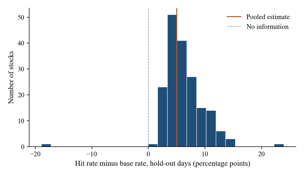
Figure 1: The hold-out difference stock by stock
Note: For each of the panel’s stocks, the hit rate minus the base rate over its events on the four hold-out days, in percentage points. The vertical lines mark zero and the pooled estimate of Table 2.
5.2 Direction and Shape
Column S1 of Table 3 reports Prediction 1 on the pooled day files. With stock-day fixed effects and time-of-day controls, the probability of an up move rises by 0.202 per unit of the reading (, 224 clusters, 14,808,739 events), an average over a relation that is steeper near zero and flatter toward the extremes (Table 4). The null of a zero coefficient is rejected under the procedure of Holm (1979) at the familywise level, and the estimate has the predicted sign, so the direction part of Prediction 1 is supported.
Table 3: Regressions of the direction of the next mid-price change
| S1 | S2 | S3 | S4 | S5 | |
|---|---|---|---|---|---|
| 0.202 | 0.180 | 0.167 | 0.183 | 0.178 | |
| (14.4) | (18.3) | (18.1) | (21.5) | (17.9) | |
| 0.113 | |||||
| (9.1) | |||||
| −0.058 | |||||
| (−3.6) | |||||
| −0.021 | |||||
| (−7.8) | |||||
| Sign of last change | −0.104 | −0.091 | −0.100 | −0.107 | |
| (−13.3) | (−11.5) | (−12.5) | (−13.2) | ||
| Sign of last change × wide spread | 0.104 | 0.090 | 0.100 | 0.106 | |
| (11.2) | (10.3) | (10.9) | (11.1) | ||
| Sign of signed volume | 0.071 | 0.070 | 0.070 | 0.070 | |
| (26.4) | (26.3) | (26.3) | (26.5) | ||
| Signed volume, scaled | 0.002 | 0.002 | 0.002 | 0.002 | |
| (2.0) | (1.8) | (2.0) | (2.0) | ||
| Spread-bucket dummies | No | Yes | Yes | Yes | Yes |
| Time-to-change dummies | No | No | No | No | Yes |
| Stock-day effects | 700 | 700 | 700 | 700 | 700 |
| Stocks (clusters) | 224 | 224 | 224 | 224 | 224 |
| Events | 14,808,739 | 14,808,739 | 14,808,739 | 14,808,739 | 14,808,739 |
Note: Linear probability models of (next mid-price change up) on the pooled day files, equation (8), with stock-day fixed effects and the dummies of thirteen time-of-day bins, one omitted. statistics in parentheses use standard errors clustered by stock with degrees of freedom. is the quoted spread in ticks, the base-ten logarithm of the stock-day’s first mid price after 09:45, and the base-ten logarithm of the time from the reading to the next change in seconds; both are centered at their sample means. A wide spread is two ticks or more. Signed volume is the aggressor-signed share volume of trades in the second before the reading, excluding those of the reading’s own book update, executions against displayed orders only, divided by its stock-day standard deviation and winsorized at five.
Table 4 and Figure 2 show the shape. The share of up moves rises across the ten bins of the reading, from 40.2% in the lowest bin to 60.8% in the highest, and the pooled share of up moves is 49.9%. The shape contrast of Section 4.3 is 0.241 (), and its null is rejected under the procedure of Holm (1979) with the predicted sign, so the plan’s shape test is supported. In Table 4 the mean readings of the two bins next to zero lie as far apart, within a hundredth of a unit of the reading, as those of each outermost pair, so the spacing does not move the contrast, and its positive sign shows that the relation flattens toward the extremes of the reading, as the shares of the outer bins in Table 4 also show. The curve pools stocks and spreads whose slopes differ (Table 5), so part of the flattening may come from that mix rather than from each stock’s own curve. The fitted independent-queue form has (standard error 0.021), and the largest gap between the fitted curve and a bin with at least 10,000 events is 6.6 percentage points. By the plan’s criterion the one-parameter form is not adequate: among the bins with at least 10,000 events, [−1.0, −0.8), [−0.8, −0.6), [+0.6, +0.8) and [+0.8, +1.0] lie more than 2 percentage points from it. The misses follow one pattern: the data are steeper than the form near zero and flatter at the extremes, a bend that one attenuation parameter cannot fit.
Table 4: Calibration of the reading
| Bin of reading | Events | Mean reading | Share up | Std. error | Fitted | Gap (pp) |
|---|---|---|---|---|---|---|
| [−1.0, −0.8) | 91,041 | −0.872 | 0.402 | 0.010 | 0.336 | 6.6 |
| [−0.8, −0.6) | 337,691 | −0.681 | 0.405 | 0.007 | 0.371 | 3.3 |
| [−0.6, −0.4) | 1,011,935 | −0.483 | 0.408 | 0.006 | 0.408 | 0.0 |
| [−0.4, −0.2) | 2,361,302 | −0.289 | 0.431 | 0.005 | 0.445 | −1.4 |
| [−0.2, 0.0) | 3,679,558 | −0.096 | 0.475 | 0.002 | 0.482 | −0.7 |
| [0.0, +0.2) | 3,663,209 | 0.096 | 0.525 | 0.002 | 0.518 | 0.7 |
| [+0.2, +0.4) | 2,317,138 | 0.288 | 0.568 | 0.005 | 0.555 | 1.3 |
| [+0.4, +0.6) | 964,276 | 0.482 | 0.595 | 0.007 | 0.592 | 0.3 |
| [+0.6, +0.8) | 303,079 | 0.679 | 0.596 | 0.008 | 0.629 | −3.3 |
| [+0.8, +1.0] | 79,510 | 0.871 | 0.608 | 0.015 | 0.663 | −5.5 |
Note: Pooled day files. The share up is the share of events in the bin whose next mid-price change is up, with a standard error clustered by stock. The fitted column is the mean over the bin’s events of , with estimated by Bernoulli maximum likelihood on all events, and the gap is the share up minus the fitted value, in percentage points. The highest bin includes a reading of exactly one.
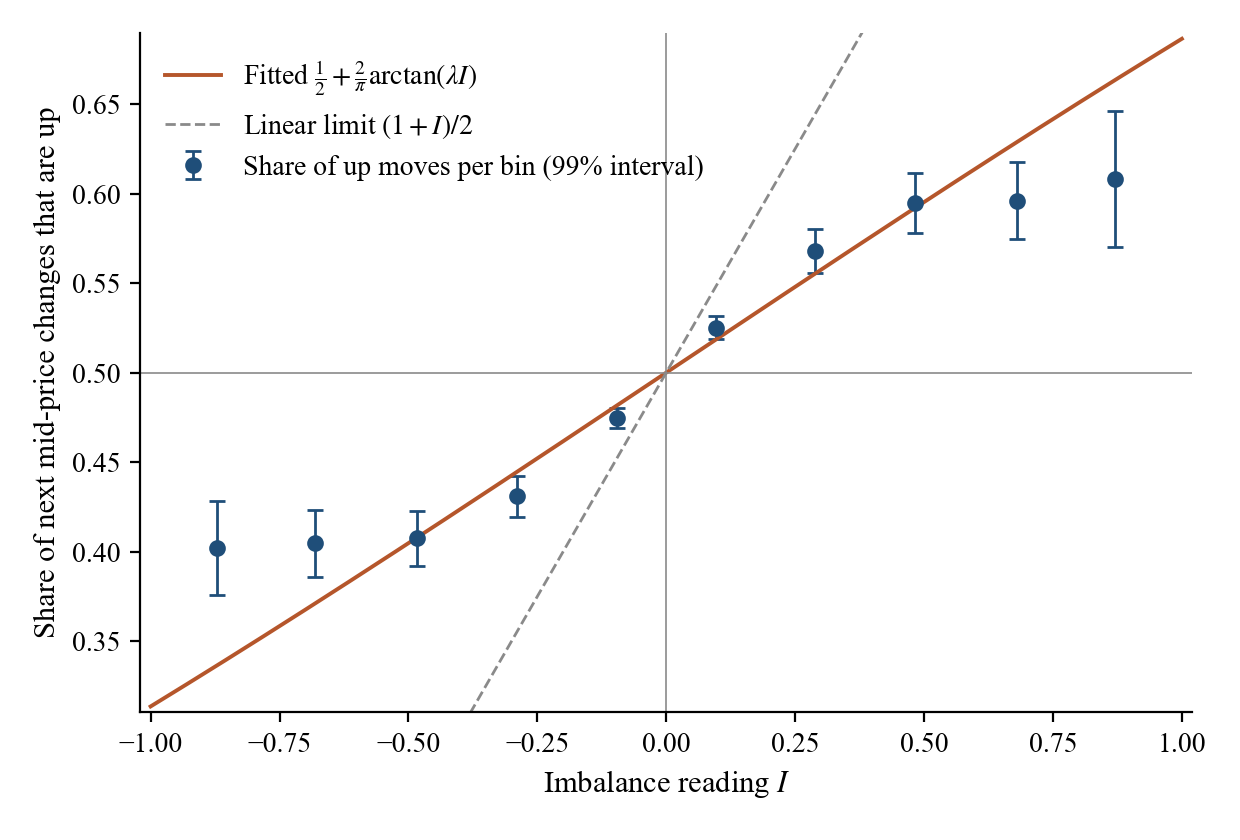
Figure 2: Calibration of the reading
Note: Points are the share of next mid-price changes that are up in each of ten bins of the reading, at the bin’s mean reading, with 99% intervals clustered by stock (Table 4). The solid curve is the fitted independent-queue form and the dashed line the linear limit of Section 2.1.
5.3 Spread and Tick Size
Column S3 of Table 3 tests Prediction 2. The interaction coefficient, the slope at a one-tick spread minus the slope at wider spreads, is 0.113 (), against a slope of 0.167 at wider spreads. The null of a zero coefficient is rejected under the procedure of Holm (1979) at the familywise level, and the estimate has the predicted sign, so Prediction 2 is supported. Panel A of Table 5 and the left panel of Figure 3 show the slope by spread bucket: it is 0.413 at one tick and 0.134 at eleven ticks or more.
Column S4 of Table 3 tests Prediction 3. The interaction coefficient, the change in the slope per tenfold increase in price, is −0.058 (), so the slope is lower for higher-priced stocks. The null of a zero coefficient is rejected under the procedure of Holm (1979) at the familywise level, and the estimate has the predicted sign, so Prediction 3 is supported. Panel B of Table 5 shows the slope by price bucket. Across the price buckets the slope is highest, and about equal, for stocks priced from twenty to one hundred dollars, and lower for both the cheaper and the dearer stocks, so the interaction describes a trend across the panel, not every bucket.
Table 5: The relation by spread, price and time to the next change
| Bucket | Events | Stocks | Hit rate | Difference (pp) | Slope | t |
|---|---|---|---|---|---|---|
| Panel A: quoted spread (ticks) | ||||||
| 1 | 2,067,519 | 224 | 59.9% | 9.91 | 0.413 | 21.9 |
| 2 | 2,928,211 | 224 | 55.8% | 5.84 | 0.261 | 13.6 |
| 3 to 5 | 3,715,327 | 221 | 54.3% | 4.32 | 0.179 | 12.4 |
| 6 to 10 | 2,342,887 | 212 | 53.9% | 3.88 | 0.153 | 12.6 |
| 11 or more | 3,754,795 | 181 | 53.8% | 3.71 | 0.134 | 10.2 |
| Panel B: stock price ($) | ||||||
| 1 to 20 | 405,436 | 40 | 55.8% | 5.84 | 0.192 | 3.5 |
| 20 to 50 | 1,839,222 | 73 | 57.3% | 7.33 | 0.284 | 12.0 |
| 50 to 100 | 3,503,184 | 82 | 56.3% | 6.34 | 0.280 | 14.2 |
| 100 to 250 | 5,622,155 | 60 | 54.6% | 4.64 | 0.186 | 8.8 |
| 250 or more | 3,438,742 | 18 | 53.8% | 3.63 | 0.134 | 8.1 |
| Panel C: time to the next change | ||||||
| Under 0.1 ms | 3,487,311 | 224 | 56.4% | 6.42 | 0.256 | 13.4 |
| 0.1 to 1 ms | 2,551,354 | 224 | 55.0% | 4.96 | 0.195 | 10.3 |
| 1 to 10 ms | 2,385,234 | 224 | 55.5% | 5.44 | 0.188 | 10.6 |
| 10 to 100 ms | 1,680,668 | 224 | 55.9% | 5.90 | 0.223 | 11.8 |
| 0.1 to 1 s | 2,408,470 | 224 | 54.7% | 4.64 | 0.183 | 11.6 |
| 1 to 30 s | 2,295,702 | 224 | 53.3% | 3.28 | 0.136 | 18.5 |
Note: Pooled day files; bucket edges fixed in the plan. The difference is the event-weighted mean of each event’s hit minus the base rate of its stock-day, computed as in Section 4.2 over all of that stock-day’s events, in percentage points. The slope is the coefficient of a regression of the outcome on the reading within the bucket, with stock-day fixed effects and no time-of-day dummies, and its statistic is clustered by stock. A bucket with fewer than 100 events is not estimated (n.a.). Estimates within buckets are descriptive.
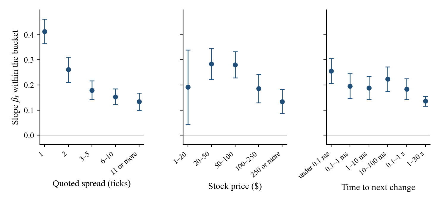
Figure 3: The slope of the reading by spread, price and time to the next change
Note: The slope of the reading within each bucket of Table 5, from a regression with stock-day fixed effects, with 99% intervals clustered by stock, from the distribution with degrees of freedom as in the tables. A bucket with too few events to estimate is left out (Table 5).
5.4 Information beyond the Last Change and Recent Trades
Column S2 of Table 3 tests Prediction 4. With the sign of the last mid-price change, its interaction with a wide spread, and the sign and size of the preceding second’s aggressor-signed volume as controls, the coefficient on the reading is 0.180 (), 89% of its value in S1. The null of a zero coefficient is rejected under the procedure of Holm (1979) at the familywise level, and the estimate has the predicted sign, so Prediction 4 is supported. Among the controls, the sign of the last change enters with a coefficient of −0.104 (), its interaction with a wide spread with 0.104 (), and the sign of the preceding second’s aggressor-signed volume with 0.071 ().
5.5 Time to Resolution
Column S5 of Table 3 tests Prediction 5. The interaction coefficient, the change in the slope per tenfold increase in the time from the reading to the next change, is −0.021 (), so the relation is weaker for changes that arrive later. The null of a zero coefficient is rejected under the procedure of Holm (1979) at the familywise level, and the estimate has the predicted sign, so Prediction 5 is supported. Panel C of Table 5 and the right panel of Figure 3 show the slope by time bucket, from 0.256 for changes within a tenth of a millisecond to 0.136 for changes after one to thirty seconds, though not at every step.
5.6 Replication across Days
Table 6 and Figure 4 report specification S1 on each day on its own. The slope is positive on each of the seven day files, with estimates from 0.179 on 2019-12-30 to 0.234 on 2019-03-27, and the null of a zero slope is rejected on every day under the procedure of Holm (1979) across the seven days. On the capture day of 2023-08-22, which the plan keeps apart, the slope is 0.244 (, 4,548,280 events), and the hold-out statistic of Section 4.2 is 6.13 percentage points over a hit rate of 56.0%.
Table 6: The slope of the reading by day
| Day | Role | Events | Stocks | Slope | Std. error | t |
|---|---|---|---|---|---|---|
| 2019-01-30 | Hold-out | 2,421,704 | 100 | 0.208 | 0.015 | 14.2 |
| 2019-03-27 | Processed earlier | 2,270,423 | 100 | 0.234 | 0.021 | 10.9 |
| 2019-07-30 | Processed earlier | 1,516,435 | 100 | 0.222 | 0.019 | 11.8 |
| 2019-08-30 | Hold-out | 1,748,447 | 100 | 0.198 | 0.021 | 9.5 |
| 2019-10-30 | Hold-out | 1,987,104 | 100 | 0.189 | 0.016 | 11.6 |
| 2019-12-30 | Hold-out | 1,564,793 | 100 | 0.179 | 0.016 | 10.9 |
| 2020-01-30 | Processed earlier | 3,299,833 | 100 | 0.196 | 0.020 | 10.0 |
| 2023-08-22 | Capture, apart | 4,548,280 | 100 | 0.244 | 0.049 | 5.0 |
Note: Specification S1 estimated on each day on its own, with stock-day fixed effects, time-of-day dummies and standard errors clustered by stock. The plan tests the seven day files together under the procedure of Holm (1979) at a familywise level of 1% and reports the capture day apart.
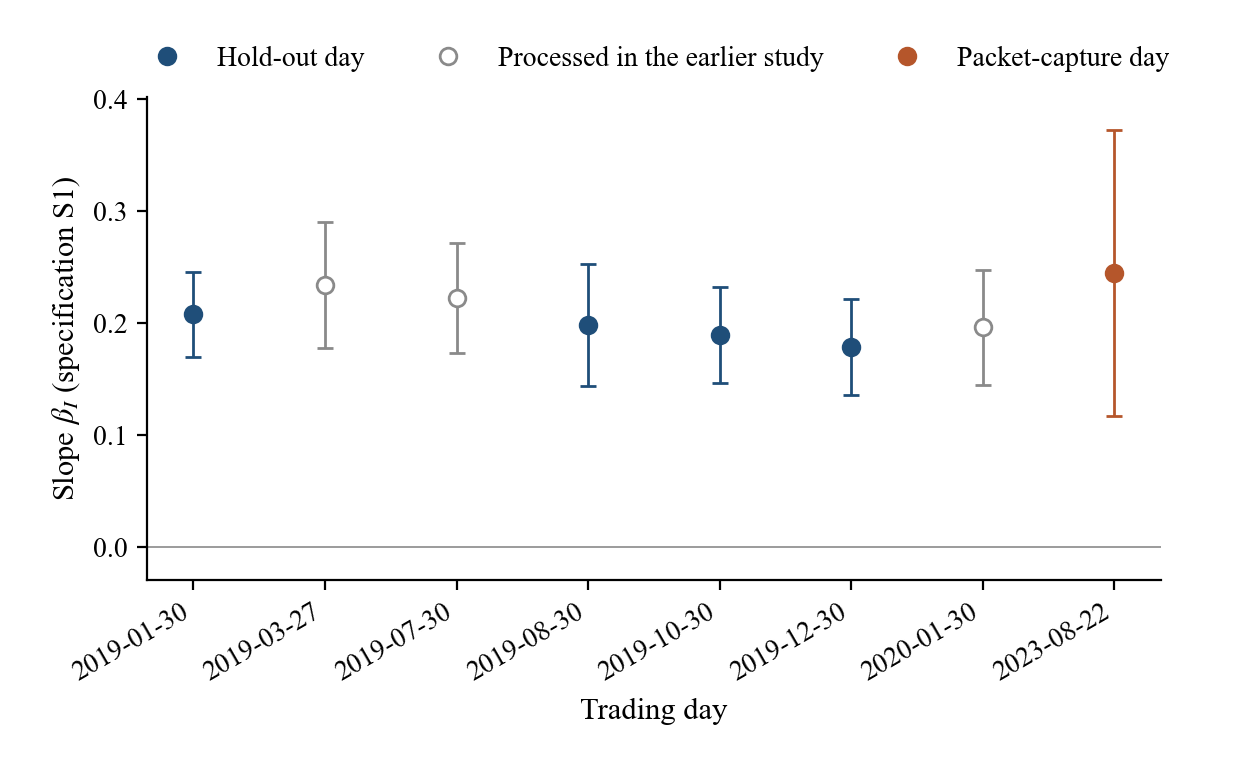
Figure 4: The slope of the reading by day
Note: The slope of specification S1 estimated on each day on its own (Table 6), with 99% intervals clustered by stock, from the distribution with degrees of freedom as in the tables. Filled markers are hold-out days, open markers the day files processed in the earlier study, and the last marker the capture day.
5.7 Robustness
The plan names no specification for its robustness checks; Table 7 reports each for specification S1, and checks (c) and (d) for S2 as well. In checks (a), (b), (d), (e), (f) and (g) of specification S1 the slope runs from 0.183 to 0.244, and every row of Table 7, the logit and the S2 rows included, keeps the positive sign and rejects a zero coefficient at the plan’s significance level.
Table 7: Robustness
| Check | Events | Stocks | Estimate | Std. error | t or z |
|---|---|---|---|---|---|
| Baseline, S1 | 14,808,739 | 224 | 0.202 | 0.014 | 14.4 |
| (a) Late readings replaced | 14,866,026 | 224 | 0.202 | 0.014 | 14.4 |
| (b) No 30-second cap | 14,866,097 | 224 | 0.201 | 0.014 | 14.5 |
| (c) Logit, S1, average marginal effect | 14,808,739 | 224 | 0.202 | n.a. | 14.0 |
| (c) Logit, S2, average marginal effect | 14,808,739 | 224 | 0.180 | n.a. | 17.8 |
| (d) Two-way clusters, S1 | 14,808,739 | 224 | 0.202 | 0.014 | 14.4 |
| (d) Two-way clusters, S2 | 14,808,739 | 224 | 0.180 | 0.010 | 18.3 |
| (e) Capture day alone | 4,548,280 | 100 | 0.244 | 0.049 | 5.0 |
| (f) Next change at least one millisecond later | 8,770,074 | 224 | 0.183 | 0.013 | 14.2 |
| (g) Without the earlier study’s stocks | 12,094,176 | 214 | 0.199 | 0.014 | 14.5 |
Note: The estimate is of specification S1, or of S2 where the row names it, except in (c), where it is the average marginal effect of the reading in a logit with stock-day intercepts estimated by full maximum likelihood; no standard error is computed for that effect (n.a.), and the statistic is the of the logit coefficient on the reading, with a standard error clustered by stock. Check (a) uses an event rule in which a later reading replaces one whose outcome came too late; (b) drops the 30-second cap; (d) clusters by stock and by day-minute (Cameron, Gelbach, and Miller (2011)); (e) is the capture day of 2023-08-22, on which the settings of the measure were selected; (f) keeps events whose next change comes at least one millisecond after the reading; (g) drops the stocks the earlier study scored. The plan names no specification for its robustness checks; each is reported for S1, and (c) and (d) also for S2. Every check except (e) uses the pooled day files.
6 Economic Magnitude and Limitations
6.1 Economic Magnitude
Table 8 sets the size of the predicted move against the cost of trading on it. Over the pooled day files the next mid-price move, signed by the reading, averages 0.186 ticks, against a mean half spread of 5.73 ticks, a ratio of 0.032. At a one-tick spread the signed move is 0.147 ticks against a half spread of 0.50. With the move in ticks as the dependent variable, the S2 slope is 0.807 (), so the expected move at a reading of one half is 0.403 ticks larger than at a reading of zero. On the four hold-out days alone the signed move is 0.181 ticks against a half spread of 5.37. A trader who crosses the spread to act on each reading therefore pays more on entry than the average move the reading predicts. The reading may still matter for decisions that do not cross the spread, such as where and when to rest passive orders and when to withdraw them, which this paper does not test.
Table 8: The size of the predicted move against the half spread
| Spread (ticks) | Events | Mean absolute move | Mean signed move | Mean half spread | Ratio |
|---|---|---|---|---|---|
| 1 | 2,067,519 | 0.620 | 0.147 | 0.500 | 0.295 |
| 2 | 2,928,211 | 0.575 | 0.087 | 1.000 | 0.087 |
| 3 to 5 | 3,715,327 | 0.724 | 0.103 | 1.897 | 0.054 |
| 6 to 10 | 2,342,887 | 1.081 | 0.161 | 3.812 | 0.042 |
| 11 or more | 3,754,795 | 2.622 | 0.383 | 17.281 | 0.022 |
| All events | 14,808,739 | 1.218 | 0.186 | 5.728 | 0.032 |
Note: Pooled day files, in ticks of one cent. The absolute move is the size of the next mid-price change; the signed move is that change multiplied by the sign of the reading, so it is positive when the reading pointed the right way; the half spread is half the quoted spread at the reading; the ratio divides the mean signed move by the mean half spread. A trader who crosses the spread to act on a reading pays the half spread on entry.
6.2 Limitations
The book and the mid price are Nasdaq’s, not the consolidated national best bid and offer, so a change on another venue that does not move the Nasdaq quotes is not an outcome here. The rates assume that the reading is acted on at its timestamp, with no display or reaction delay (Section 3.1), and 40.8% of next changes arrive within one millisecond of the reading; robustness check (f), which keeps only the events whose next change comes later, gives a slope of 0.183, and its null of zero is rejected at the plan’s significance level with a positive sign. The sample covers seven days between January 2019 and January 2020 and the capture day of 2023-08-22, and its stocks are the most active Nasdaq-listed common stocks, so the results describe active stocks in that period. The settings of the measure were selected on the capture day, so that day’s results are not out of sample. We study the measure in the settings the plan fixes and do not compare it with other weightings or numbers of levels. Predictions 2 and 3 are tests of the measure: its weighting of the levels beyond the best quote changes with the median spread in ticks, so part of the variation they find may come from the reading rather than from the race (Section 2.5). The signed-volume control of Prediction 4 counts executions against displayed orders only. The linear probability model is a summary of a nonlinear relation, and robustness check (c) gives the logit counterpart. The shape contrast of Prediction 1 uses the nominal width of the bins; it reads as curvature here because the mean readings of the bins it uses are spaced alike (Section 5.2). The calibration of Table 4 shows that the one-parameter form of Section 2 does not fit every bin of the reading within the plan’s band. VisualHFT builds and sells the application whose measure we study. The plan and the estimation code were fixed before any panel result was computed, and Appendix A.3 lists the commits made after that. Every result the plan names is reported, except that the shares of events the event rule changes are reported per day rather than per stock-day (Table A1).
7 Conclusion
The imbalance of the visible order book, as a commercial order book visualization application computes it in the settings tested here, predicts the direction of the next mid-price change on active Nasdaq-listed stocks on days held out before the analysis. Under a plan fixed before the outcomes of the hold-out days were computed, its sign matched the next change 55.1% of the time on those days, against a base rate of 50.0%. The relation is stronger at a one-tick spread, for lower-priced stocks and for mid-price changes that arrive soonest, as predicted, and it survives controls for the last mid-price change and recent signed volume. For a trader the reading is information about the direction of the next mid-price change, and on the hold-out days its average move signed by the reading is smaller than the half spread paid to cross on entry.
References
- Avellaneda, Marco, Josh Reed, and Sasha Stoikov, 2011, Forecasting prices from Level-I quotes in the presence of hidden liquidity, Algorithmic Finance 1, 35–43.
- Cameron, A. Colin, Jonah B. Gelbach, and Douglas L. Miller, 2011, Robust inference with multiway clustering, Journal of Business & Economic Statistics 29, 238–249.
- Cao, Charles, Oliver Hansch, and Xiaoxin Wang, 2009, The information content of an open limit-order book, Journal of Futures Markets 29, 16–41.
- Cartea, Álvaro, Ryan Donnelly, and Sebastian Jaimungal, 2018, Enhancing trading strategies with order book signals, Applied Mathematical Finance 25, 1–35.
- Cont, Rama, and Adrien de Larrard, 2013, Price dynamics in a Markovian limit order market, SIAM Journal on Financial Mathematics 4, 1–25.
- Cont, Rama, Arseniy Kukanov, and Sasha Stoikov, 2014, The price impact of order book events, Journal of Financial Econometrics 12, 47–88.
- Gould, Martin D., and Julius Bonart, 2016, Queue imbalance as a one-tick-ahead price predictor in a limit order book, Market Microstructure and Liquidity 2, 1650006.
- Holm, Sture, 1979, A simple sequentially rejective multiple test procedure, Scandinavian Journal of Statistics 6, 65–70.
- Jain, Raj, and Imrich Chlamtac, 1985, The P² algorithm for dynamic calculation of quantiles and histograms without storing observations, Communications of the ACM 28, 1076–1085.
- Nasdaq, 2023, Nasdaq TotalView-ITCH 5.0, technical specification, revision of April 28, 2023, The Nasdaq Stock Market LLC.
- Petersen, Mitchell A., 2009, Estimating standard errors in finance panel data sets: Comparing approaches, Review of Financial Studies 22, 435–480.
- Stoikov, Sasha, 2018, The micro-price: A high-frequency estimator of future prices, Quantitative Finance 18, 1959–1966.
Appendix A: Data, Code and Reproducibility
A.1 Data
The seven day files are Nasdaq’s public TotalView-ITCH sample files; their names and sizes in bytes below match the directory listing of emi.nasdaq.com read on 2026-11-09. The capture day is a set of 103 packet-capture files of the same feed for 2023-08-22, held by VisualHFT and named by their start time; it is not one of the public sample files.
Seven day files (Nasdaq public sample directory, emi.nasdaq.com, ITCH/Nasdaq ITCH), size in bytes:
  01302019.NASDAQ_ITCH50.gz   4764426091   2019-01-30   hold-out
  03272019.NASDAQ_ITCH50.gz   5510131732   2019-03-27   processed in the earlier study
  07302019.NASDAQ_ITCH50.gz   3662140094   2019-07-30   processed in the earlier study
  08302019.NASDAQ_ITCH50.gz   4075649457   2019-08-30   hold-out
  10302019.NASDAQ_ITCH50.gz   3872931242   2019-10-30   hold-out
  12302019.NASDAQ_ITCH50.gz   3524013057   2019-12-30   hold-out
  01302020.NASDAQ_ITCH50.gz   5597158940   2020-01-30   processed in the earlier study
Capture day 2023-08-22, 103 files, named by their start time:
  ny4-xnas-tvitch-a-20230822T000000.pcap, then
  ny4-xnas-tvitch-a-20230822T070000.pcap ... ny4-xnas-tvitch-a-20230822T235000.pcap
Table A1 reports the panel and the event rules for each day.
Table A1: Panel construction and event rules by day
| Day | Replayed | Panel | Lowest rank used | Events | Dropped share | Replaced share, rule (a) | Extra events without cap |
|---|---|---|---|---|---|---|---|
| 2019-01-30 | 120 | 100 | 100 | 2,421,704 | 0.31% | 0.30% | 7,414 |
| 2019-03-27 | 120 | 100 | 101 | 2,270,423 | 0.25% | 0.25% | 5,606 |
| 2019-07-30 | 120 | 100 | 100 | 1,516,435 | 0.62% | 0.62% | 9,407 |
| 2019-08-30 | 120 | 100 | 100 | 1,748,447 | 0.53% | 0.53% | 9,359 |
| 2019-10-30 | 120 | 100 | 100 | 1,987,104 | 0.43% | 0.43% | 8,614 |
| 2019-12-30 | 120 | 100 | 102 | 1,564,793 | 0.67% | 0.67% | 10,502 |
| 2020-01-30 | 120 | 100 | 101 | 3,299,833 | 0.20% | 0.20% | 6,456 |
| 2023-08-22 | 120 | 100 | 100 | 4,548,280 | 0.19% | 0.19% | 8,609 |
Note: Replayed is the number of top-ranked eligible stocks replayed, panel the number kept after the exclusions of Section 3.2, and lowest rank used the rank of the last stock kept. Events are the events of Section 4.1; the dropped share is the share of intervals whose first reading was dropped because the next change came too late; the replaced share is the share of intervals in which rule (a) of Section 4.5 would have used a later reading instead; the extra events are those the rule without the 30-second cap adds. The plan names the two shares per stock-day; they are reported here per day.
A.2 Pre-Analysis Plan
The plan was committed on 2026-11-09 to a repository held by VisualHFT, together with the list of replayed stocks for each day. No day had been replayed for this study when it was committed, and its amendment log is empty. The plan fixes the measure’s settings from the earlier study’s selection on 2023-08-22 (Section 3.3); that study’s results are kept on record and are not part of this paper. The plan’s hash and commit are printed below with those of the analysis code and the application build.
Pre-analysis plan, sha256     d551fdd8e2cca2fec3cf3d62f6fff6c0c08afbf9d18d3643f2ebbd4950bfb83d
Pre-analysis plan, commit     e09e1b1f8f3545092c49fd50d9f7b502cb5496f4
Analysis code, commit         1cfc0e321ad1ebf45ea6370bf6a878dee3bfb4ab
Application build, commit     d45defc79aefcf2d98de8af2545f6bfe4653642e
Replay program, sha256        8c41ba83cf2a58d027eaf60b2b6b74ff50ef86e85eb6a0f1d147956e5df7af27
A.3 Code and Build
The extraction, event and analysis code was committed as e53b40f2e before any panel result existed, with its tests. Three commits changed it before the reported numbers were computed. Commit 69e9713ea made the extractor read the key under which a run with a single aggregation setting writes the measure, after the first day’s extraction had returned no readings; no event or result existed before it. Commit c9031204e adds each regression coefficient to the output under its regressor’s name, and commit 1cfc0e321 reads the code’s provenance from the repository root; neither changes an estimate, a sample, an event rule or a test. Between those two commits, at 02:19 on 2026-11-09, a test run of the analysis on the first replayed day, 2019-01-30, which is a hold-out day, produced every statistic and the classification for that day alone; it was run to check the pipeline end to end, and no part of the plan, the event rule, the specifications or the estimation code changed after it. Every reported number was computed by the analysis code commit printed in Section A.2, with no uncommitted change in the analysis code.
Every day was replayed with one build of the application and one build of the replay program, both printed in Section A.2. The replay program records that the repository held uncommitted changes when it ran on four of the eight days; they were documentation and paper tooling, and no source or project file of the application differs from the build commit in the repository or in the working tree. The look at GLNG in Section 5.1 was made after the analysis, outside the plan, with a separate script on the stored events of 2019-08-30; it changes no estimate, sample or test.
The measure’s code is open source. The three files that compute it, ImbalanceCalculator.cs (equation (7)), SpreadScaleResolver.cs (the scale ) and P2Quantile.cs (the running median of the spread), are in the folder VisualHFT.Plugins/Studies.LOBImbalance/Model of the public repository github.com/visualHFT/VisualHFT, and on November 9, 2026 they were identical to those of the build used here. The replay program, the analysis code and the pre-analysis plan are held by VisualHFT and are available to researchers on request; the hashes and commits of Section A.2 identify the versions used.
A.4 Classification
VisualHFT Research classifies each tested measure in one of three classes. The strongest requires that the pre-registered hold-out test pass pooled and on each hold-out day, that Prediction 4 be supported, and that the mean next move signed by the reading exceed the mean half spread on the hold-out days; the middle class requires that the direction test of Prediction 1 be supported; a measure that meets neither is in the weakest class. The rule was committed with the analysis code before any panel result existed, and it uses the pooled direction test of Prediction 1 only, not the plan’s per-day rule of Section 4.4. This paper’s evidence is classified MECHANISM, the middle class, because the pooled direction test of Prediction 1 is supported; it is not in the strongest class because the mean signed move is 0.034 times the mean half spread on the hold-out days (Section 6.1).
A.5 Change Log
Version 1, dated November 8, 2026, was an internal draft built on the earlier 14-stock study and was never published. Version 2, dated November 9, 2026, replaces it with the pre-registered panel study reported here, in the working-paper format. A research note on the VisualHFT website dated October 19, 2026 reported order book imbalance results from the earlier study; those results are superseded by this paper.
Appendix B: The Measure in VisualHFT
B.1 Where the Measure Lives
The measure is the LOB Imbalance study, one of the study plug-ins of the VisualHFT application. A user adds the study for one data provider and one symbol; it plots the reading and the market mid price on one chart and shows the latest reading on a tile. The panel of this paper ran the same study code, unchanged, in a replay program that links the application’s TotalView-ITCH parser and order book and runs the study’s output queue inline on the replay thread, where the application runs it on a thread of its own.
B.2 Settings That Reproduce the Tested Form
Figure B1 shows the study’s settings window, where the tested form is the weighting Touch Weighted with No Aggregation. The number of book levels is a setting of the data connector rather than of the study, and Figure B2 shows it at ten in the replay connector’s Depth Levels field. These settings are not the study’s defaults (Section 3.3); the Touch Weighted weighting has been in every release of the application since release 0.1.16.
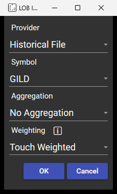
Figure B1: The study’s settings in VisualHFT
Note: Provider, symbol, aggregation and weighting of the LOB Imbalance study, set as tested.
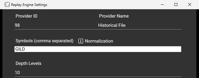
Figure B2: The number of book levels in VisualHFT
Note: The replay connector’s settings for a TotalView-ITCH file, with ten book levels per side.
B.3 Reading the Display
A reading above zero means more distance-weighted size on the bid side than on the ask side, and a reading below zero the reverse. On the hold-out days the median absolute reading was 0.206, and Table 4 shows how the share of up moves varies with the reading. The chart draws each reading until the next one, beside the mid price, so a lean that holds can be seen before the quote moves.
B.4 Companion Views
Figure B3 shows the order book ladder of the Book Viewer Desk, ten price levels per side, the levels the reading weighs. Figure B4 shows the Book Toxicity Desk, where the study’s tile sits beside the application’s order-flow studies.
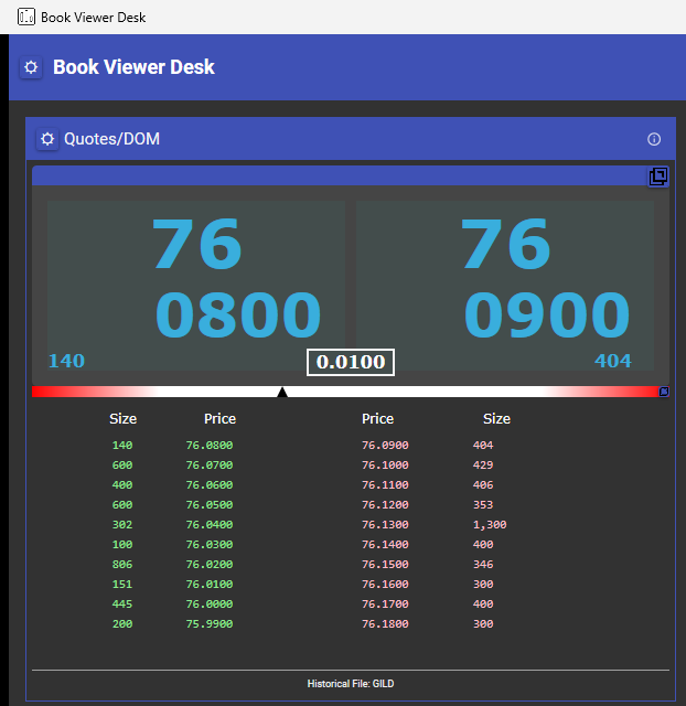
Figure B3: The Book Viewer Desk in VisualHFT
Note: The order book ladder for GILD on the capture day, with the best bid and ask above it; the still is cropped above the Desk’s row of tiles.
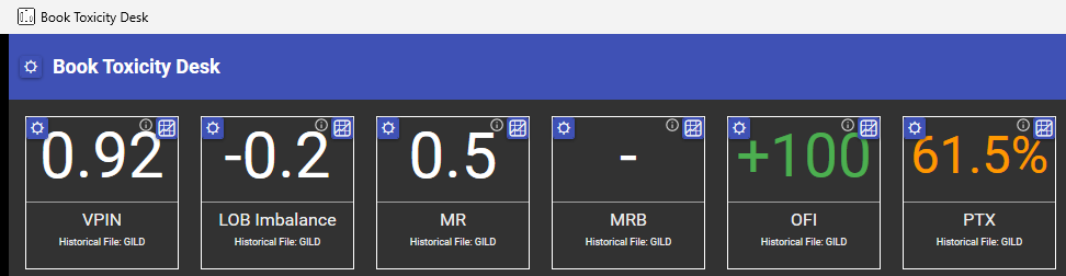
Figure B4: The Book Toxicity Desk in VisualHFT
Note: The study’s tile beside the application’s other order-flow tiles, for GILD on the capture day.
B.5 Captured Examples
Figures B5, B6 and B7 come from screen recordings of the application replaying the capture day, 2023-08-22, at the tested settings; the PDF prints a still of each, and the version of this paper at visualhft.com/research/lob-imbalance plays the recordings. They were selected among moments in which the reading held one sign and the mid price then ran in its direction, ranked first by whether that run reached two ticks and then by the size of the lean and of the move, so they show correct calls and are not a random sample. The two GILD recordings were made with the replay at one tenth of real time, with the stretches that hold no mid-price change fast-forwarded, and the CSCO recording at real time. On that day, across the panel, the sign of the first new reading after each mid-price change, the event of Section 4.1, matched the next change 56.0% of the time against a base rate of 49.9%; the figures show leans held for seconds, which that rate does not measure. The labels, boxes, captions and speed badges drawn over the application in the stills and the recordings are annotations added to the recording.
Figure B5: GILD, an upward lean followed by a rise
Note: From 14:35:40.637 ET the reading held above zero for 3.9 seconds, at a time-weighted +0.17. At 14:35:44.678 ET the bid and the ask rose, and the mid price rose 3 ticks by 14:35:45.153 ET, at a one-tick spread.
Figure B6: GILD, a downward lean followed by a fall
Note: From 15:24:46.635 ET the reading held below zero for 3.7 seconds, at a time-weighted −0.16. At 15:24:50.418 ET the bid and the ask fell, and the mid price fell 2 ticks, at a one-tick spread.
Figure B7: CSCO, a downward lean followed by a fall
Note: From 13:33:41.357 ET the reading held below zero for 23.2 seconds, at a time-weighted −0.18. The first mid-price change, a half tick down at 13:34:05.289 ET, reversed within a tenth of a millisecond, and at 13:34:06.741 ET the bid and the ask fell one tick.